Felix Kleinert – IntelliAQ

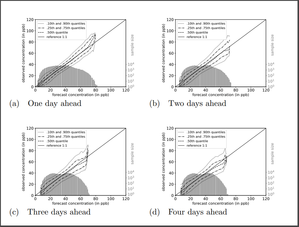
Human beings, animals and crops are directly exposed to the ambient airmass of the lower part of the atmosphere (planetary boundary layer). This airmass may contain several pollutants like ozone which is harmful to living beings (WHO, 2013; Bell et al., 2014; Lefohn et al., 2017; Fleming et al., 2018 ) and certain crops (Avnery et al., 2011; Mills et al., 2018). Therefore, the prediction of ozone concentrations is of significant importance to issue warnings for the public if high ozone concentrations are foreseeable.

We develop deep neural networks to predict near-surface ozone concentrations for more than 300 German measurement sites. Our recent model consists of multiple convolutional layers which we group into individual inception blocks (extension of Szegedy, 2015). Each inception block consists of three convolutional, and two pooling towers (max, mean) [Figure 6]. We use chemical precursors and meteorological variables of the seven previous days as input to predict the daily maximum eight-hour average (dma8eu) for a lead time of up to four days.

We create a workflow which ensures that the full workflow, including downloading the data, preprocessing, training, and postprocessing steps, is reproducible.

Figure 7:Inception block with dimensionality reduction and batch normalisation before activation. Successive layers are grouped to towers. The input and output layer of an inception block are colour coded in green, pooling layers in red, filter reduction layers

References:
WHO, 2013: http://www.euro.who.int/en/health-topics/environment-and-health/air-quality/publications/2013/health-risks-of-air-pollution-in-europe-hrapie-project.-recommendations-for-concentrationresponse-functions-for-costbenefit-analysis-of-particulate-matter,-ozone-and-nitrogen-dioxide
Bell et al., Who is More Affected by Ozone Pollution? A Systematic Review and Meta-Analysis, 2014: https://doi.org/10.1093/aje/kwu115
Lefohn et al., Responses of human health and vegetation exposure metrics to changes in ozone concentration distributions in the European Union, United States, and China, 2017: https://doi.org/10.1016/j.atmosenv.2016.12.025
Fleming et al., Tropospheric Ozone Assessment Report: Present-day ozone distribution and trends relevant to human health, 2018: https://doi.org/10.1525/elementa.273
Avnery et al., Global crop yield reductions due to surface ozone exposure: 1. Year 2000 crop production losses and economic damage, 2011; https://doi.org/10.1016/j.atmosenv.2010.11.045
Mills et al., Ozone pollution will compromise efforts to increase global wheat production, 2018: https://doi.org/10.1111/gcb.14157
Szegedy et al., Going deeper with convolutions, 2015: https://doi.org/10.1109/CVPR.2015.7298594

To evaluate the model performance, we base our analysis on the full joint distribution of forecasts and observations (Murphy and Winkler, 1987). We access detailed information on the joint distribution by factorisation into a conditional, and a marginal distribution [Figure 10].

Moreover, we evaluate our model against persistence and a climatological (observational) reference model. A new model only has a genuine added value against those simple reference models, if it outperforms both of them. To analyses this, we use skill scores which are relative relations of scoring rules like the mean squared error (MSE).

Figure 11: Conditional quantile plot for lead time up to four days ((a) to (d)). Conditional percentiles (.10th and .90th, .25th and .75th and .50th) from the conditional distribution p(o|m) are shown as lines in different styles. The reference line indicates a hypothetic perfect forecast. The marginal distribution of the forecast p(m) is shown as log-histogram.

Author: Felix Kleinert

Near surface ozone predictions

Statistics